|
About 2 years ago I was discussing New Zealand climate with a way-more-senior-than-me colleague and they asked me about 'Kidson types' and to be honest I'd never heard of them. Now, if you ask most people about them, or read about them in recent papers, you'll be referred to this paper, which I'll call K2K from now on... 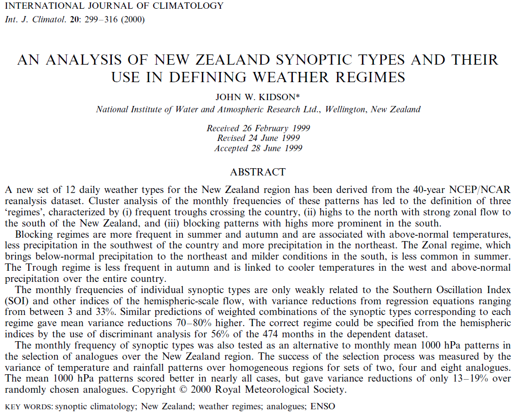 In (very) brief, the so-called Kidson types are 12 maps of 1000hPa geopotential height - basically the same as mean sea level pressure - which encapsulate the main weather types which New Zealand experiences. The next figure shows what they look like (replotted in Ackerley et al., 2011)... 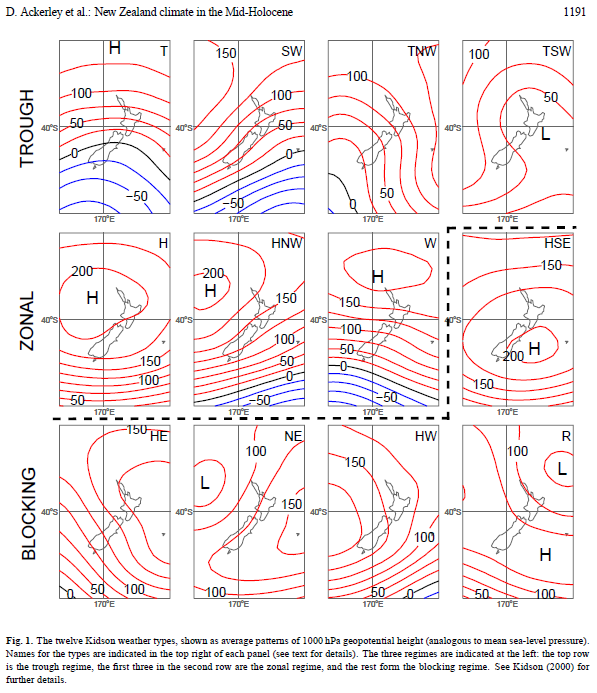 Now I don't intend to go too far into the precise scientific details of these types but you can get a good idea of the weather types associated with each of them by noting that - in the southern hemisphere - weather systems rotate clockwise round low pressure systems and anticlockwise around highs. 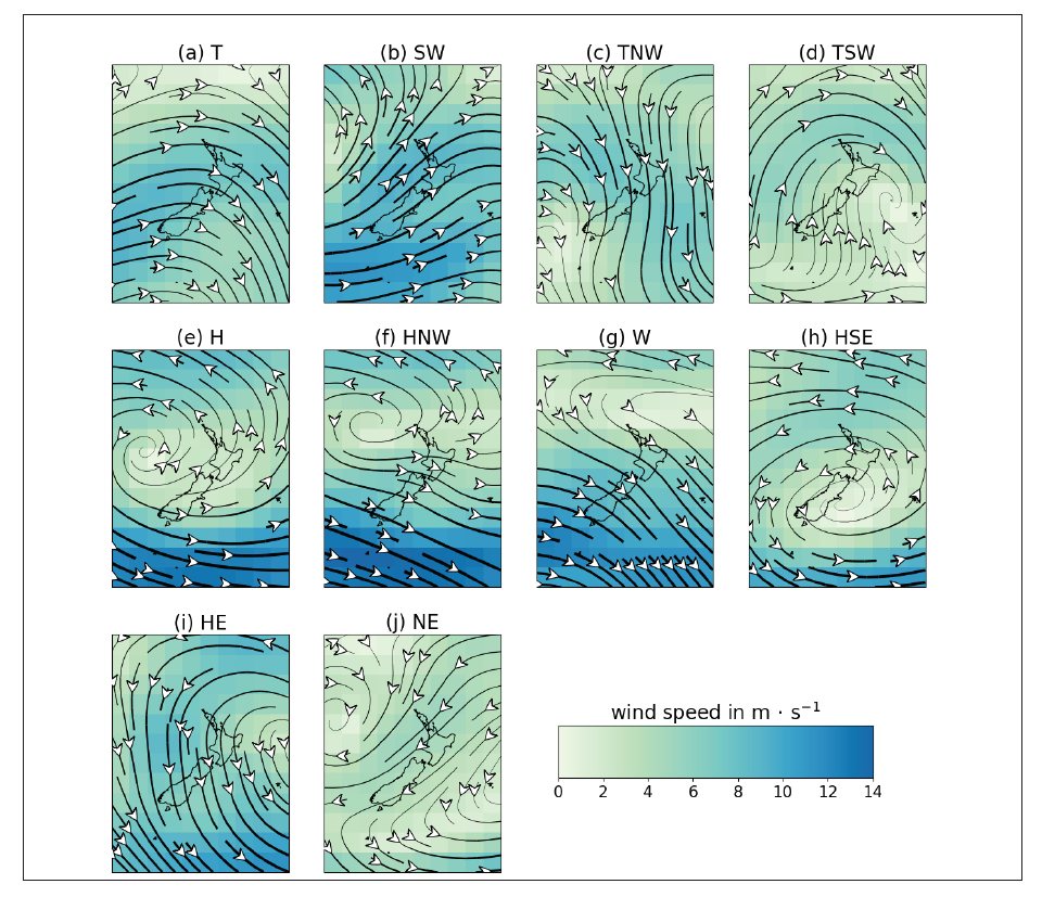 What I hope to achieve in this post is to illustrate that it's OK not to understand something and that it's OK to ask a lot of questions.  When I first read K2K, I was pretty baffled. It was the first paper I'd read on synoptic - think 'about 1000km in size'- weather types. This is normal for getting into any new area of science I know but there was one thing which really got me; how are the 12 weather types actually generated mathematically. One thing which was apparent to me from the wider literature was the following:
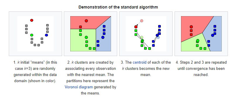
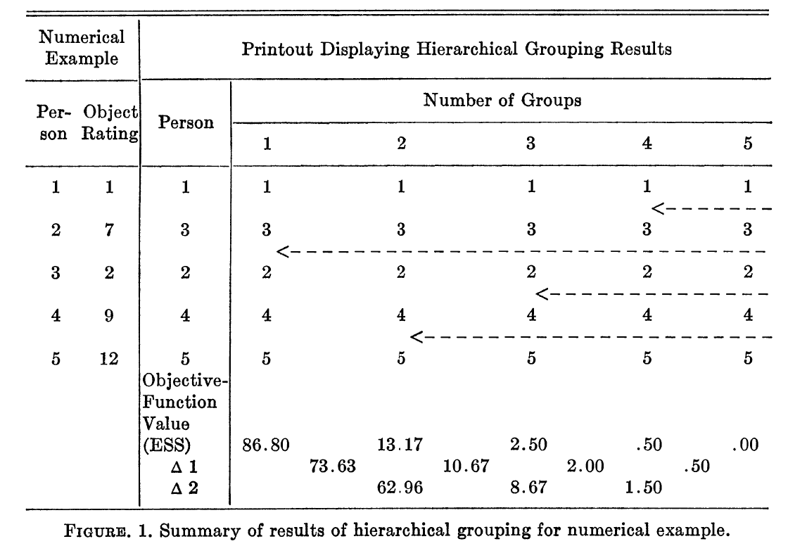 Aaaaaaaanyway, the point I'm trying to make here is that - yes OK - many people are familiar with clustering techniques but I wasn't, and trying to find out exactly how the maps above were generated was starting to drive me around the bend. At this point I was pointed in the direction of an online notebook by my Colleague Nicolas Fauchereau...  Along with a couple of helpful chats with another colleague (Drew Lorrey) on more general aspects of clustering techniques and their uses, advantages and limitations, this notebook gave me a massive step-up in getting to the bottom of my problem. However, Nicolas' notebook shows exactly the type of problem that I was coming up against; the K2K was not clear... 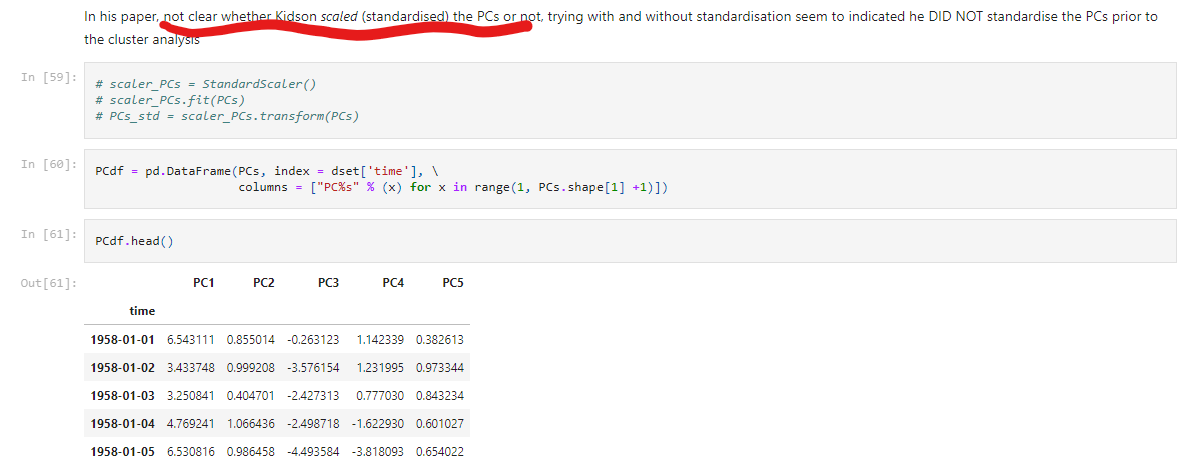 By this point, I knew that the basic procedure to generate the weather types was as follows:
 Luckily nowadays, there are Python packages for everything and from the notebook above I learnt about the scikit-learn package which can be used for the k-means clustering bit. Also, luckily for me as a user of the Iris package for working with geospatial data, there is the eofs package written to cater for the 'cubes' of data which Iris requires... 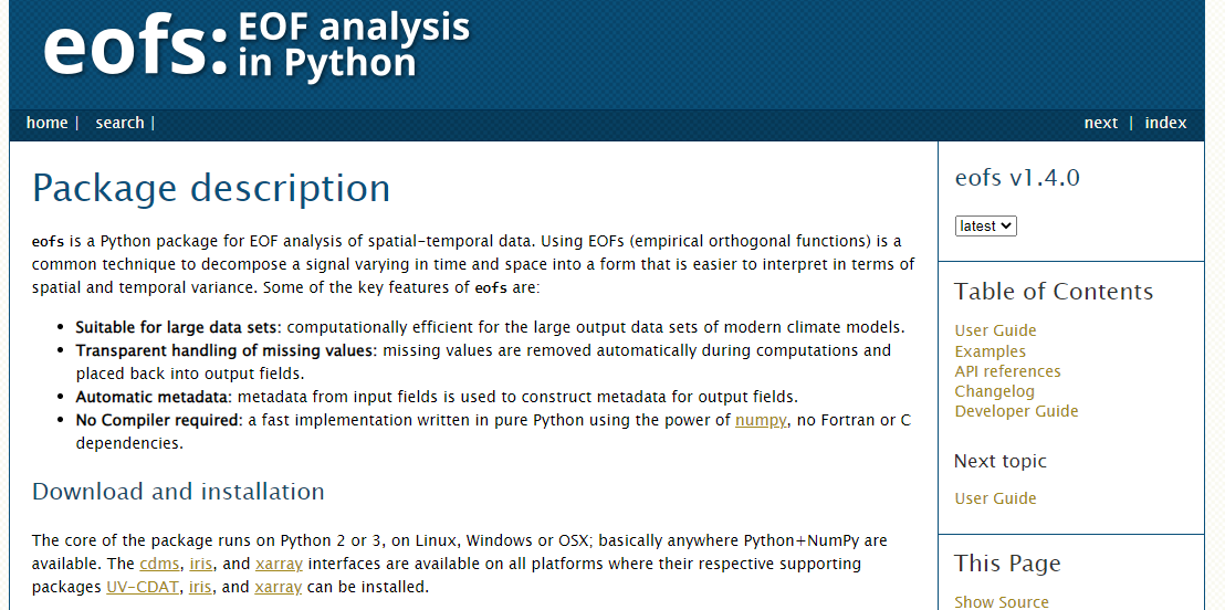 Now at this point, I was able to start my first proper task; to reproduce the Kidson types as obtained in K2K and plotted above. This proved to be significantly more challenging than I had anticipated. This was partly because of me being a noob in this field but also because the lack of detailed information on precisely how the types themselves were generated. At this point, James Renwick enters the story and after a couple of meetings and many emails, I finally managed to get my head around the problem at hand. We're lucky nowadays that online code repositories exist and I have put all my code relating this on my GitHub. 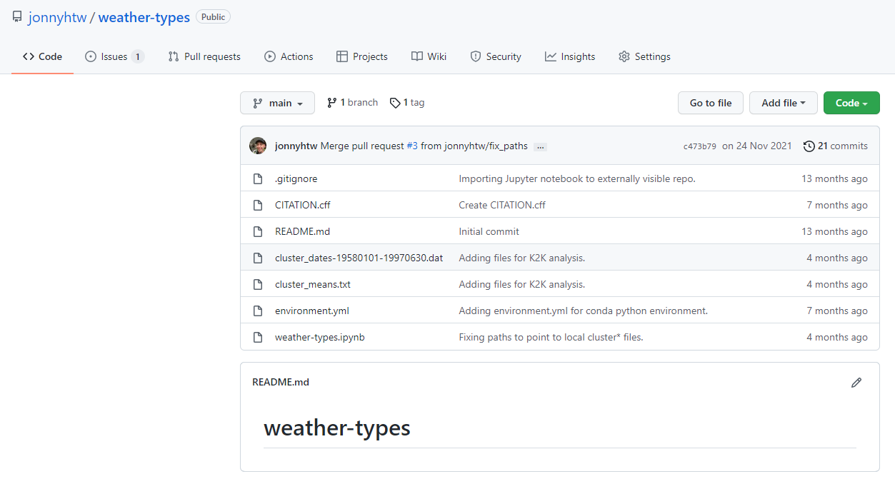 I also included an appendix in the paper which I wrote with James which I hope will be of use to future researchers in this area. I would have saved - I reckon - about a month by having had access to something like this in the first place. 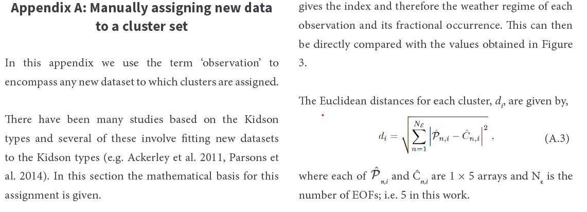 This paper turned into a bit of a labour of frustration at some points but ultimately I hope that I have provided a useful resource for future researchers who want to understand how the types themselves are generated but are stymied by the lack of detailed information on how the types themselves are actually generated. There seemed to be a pervasive assumption that 'everyone knew' how these types were generated whilst at the same time, no-one could actually point me a method of exactly how this was done. Finally, and perhaps most usefully to others, was the suggestion by the peer-reviewers that we should include new weather types from the ERA5 reanalysis, must more up to date and higher resolution than the original NCEP/NCAR one used in K2K, and here they are... 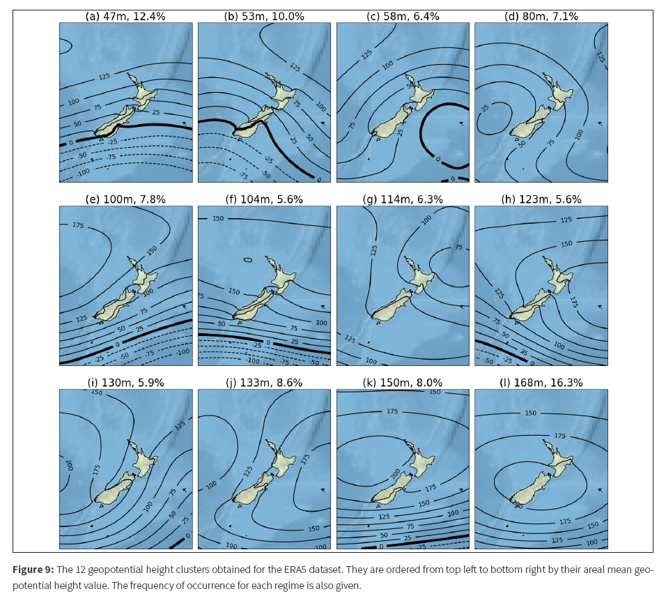
0 Comments
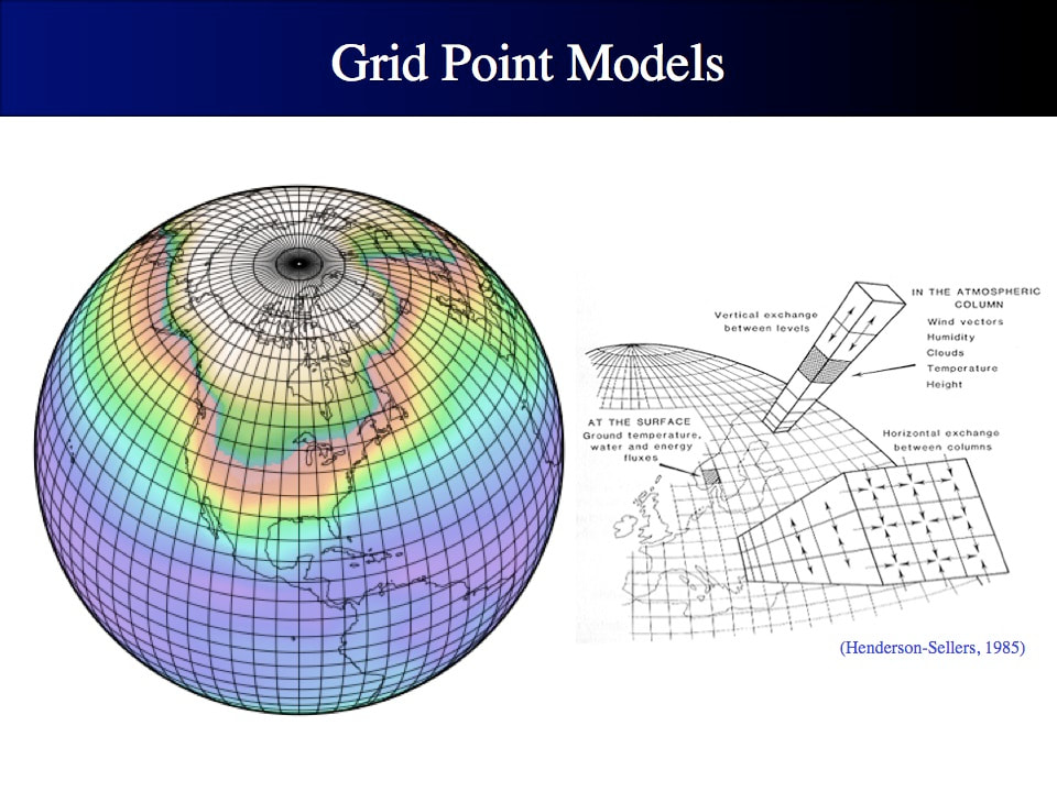 Many climate and earth system models cover the whole world, including the New Zealand Earth System Model (NZESM). Due to their global scale, the grid scales used by these models tend to be fairly coarse. In the NZESM for example, the atmosphere grid uses the so-called 'N96' scale, which is of the order 100km. This figure shows an example monthly mean near-surface specific humidity for the NZESM. 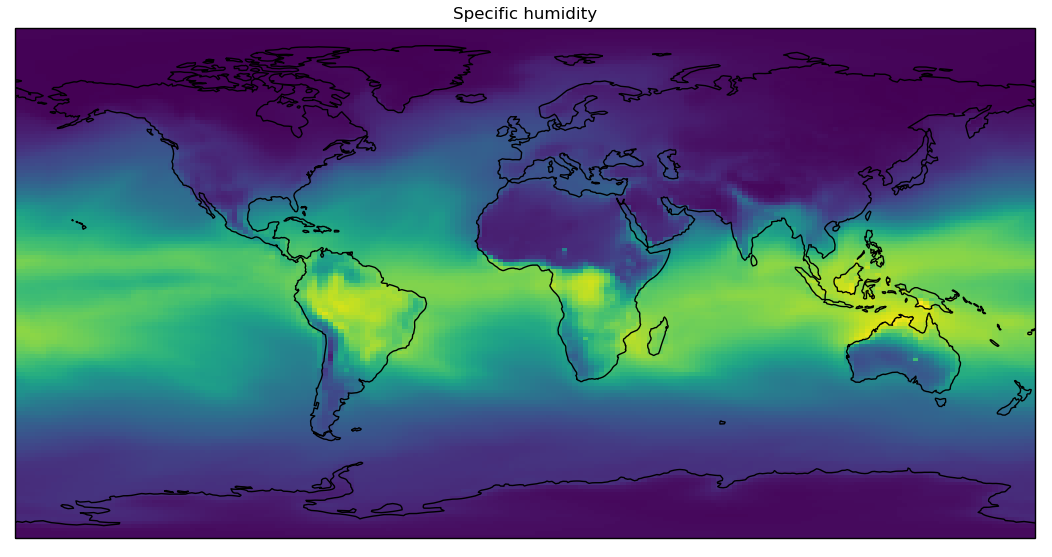 On this global scale, it is not immediately obvious that the grid is fairly coarse so let's look at Aotearoa New Zealand close up... 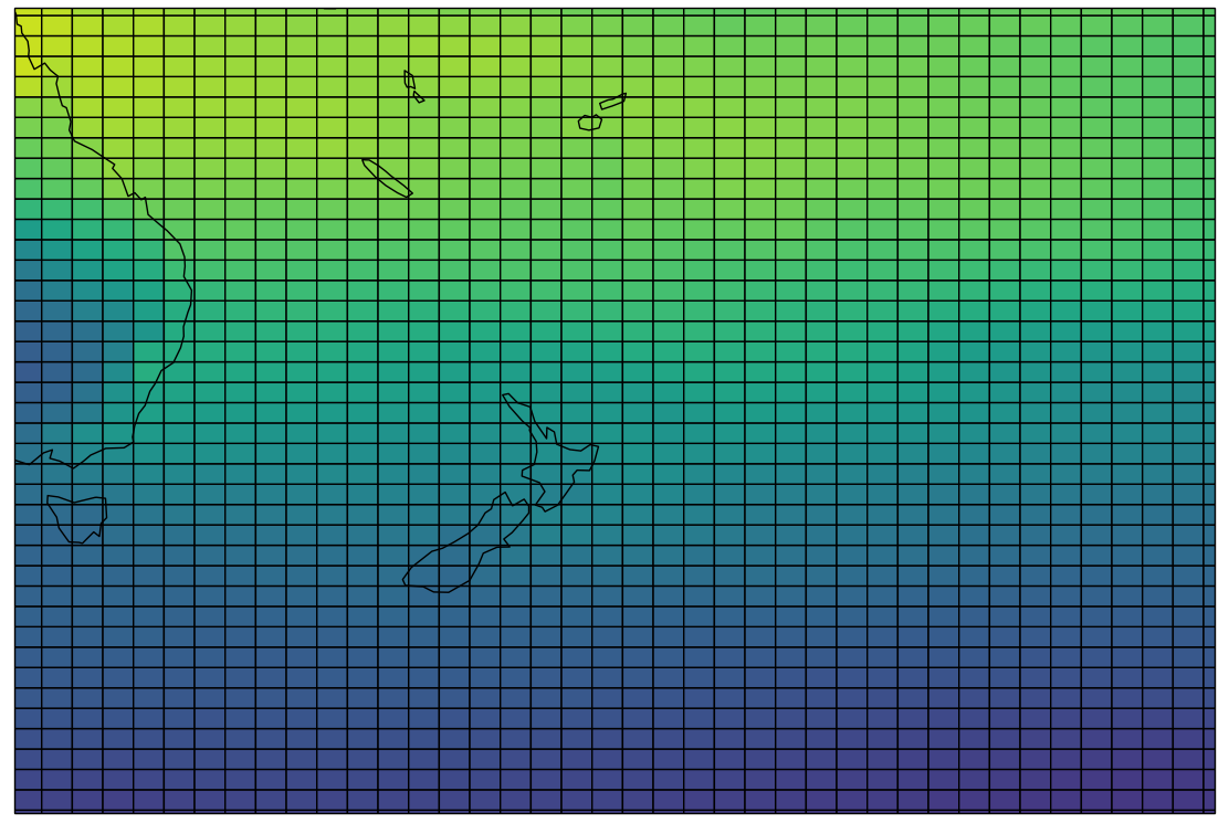 As you can see from this, the gridscale is very roughly the size of a 'region' of the country, like Waikato or Northland; as a rule of thumb. In addition you can't use individual grid boxes for projections! Now one thing which is really great about this coarse grid is that you can include a wide variety of model complexity; this is really the definition of an 'earth system' model as compared to a 'climate' model. The GENIE model has a great figure that represents the level of complexity present in the NZESM nicely... 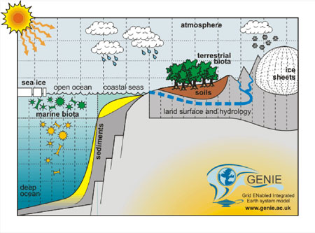 So in summary, in order to get any information on finer scales than individual NZ regions, you need to use a different model. This is exactly the basis of this project within the Deep South National Science Challenge... 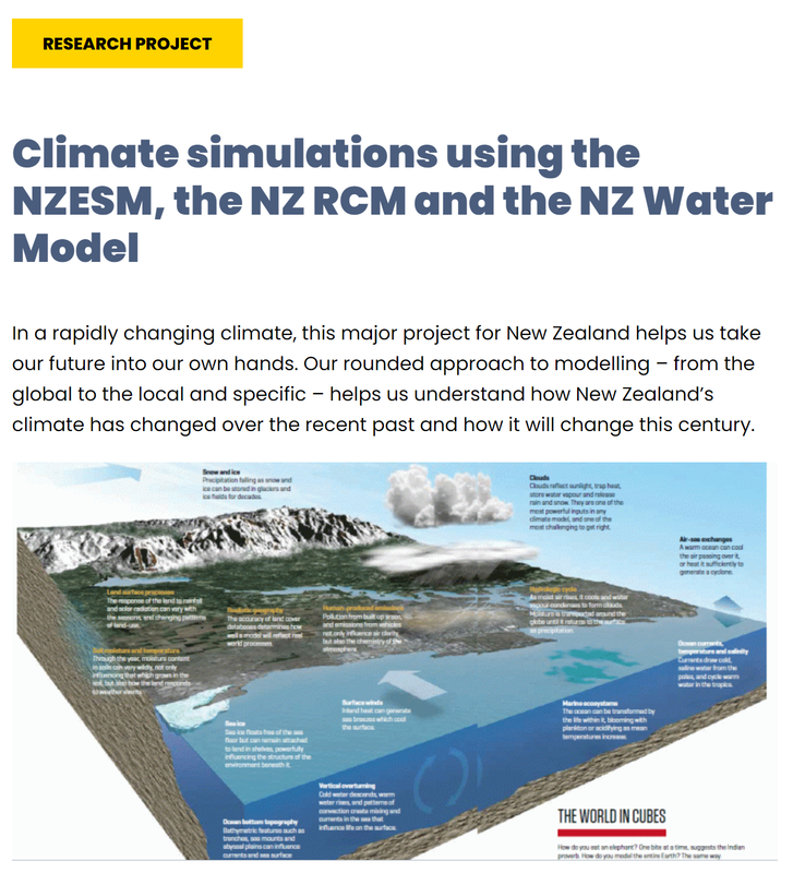 You can find out more about this project here. This project involved three inter-related but different models:
Crucially, this modelling chain is, well, exactly that; a chain! The output of the NZESM is fed into the regional atmosphere model, producing data like rainfall intensity at a significantly higher resolution. This higher-resolution atmosphere data can then be fed directly into the hydrological model producing internally-consistent projections at various scales. This figure shows the resolution of the NZRCM (from Stephen Stuart, NIWA). 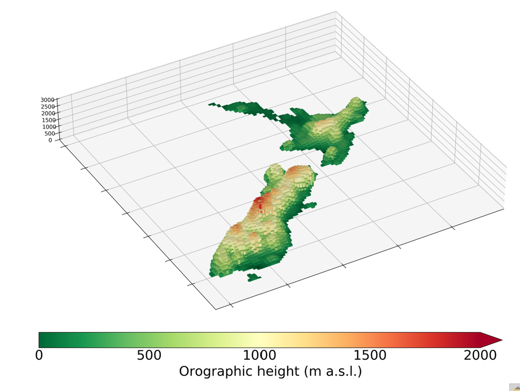 In this depiction of the RCM, the gridscale is much finer, representing features like Rakiura Stewart Island, and the Hauraki Gulf. At the length scales characteristic of the RCM, modellers are able to represent features which are absent in the global model. An example of the features present in the RCM is the Southern Alps. 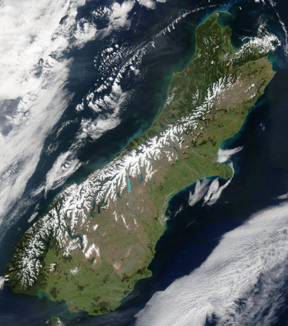 This huge mountain range spanning the entire South Island greatly influences rainfall, particularly in the West Coast region. Simulations using the RCM forced by data from the global NZESM are being run as I write! What about our river catchments though. Here's a NIWA map of some of the bigger ones... 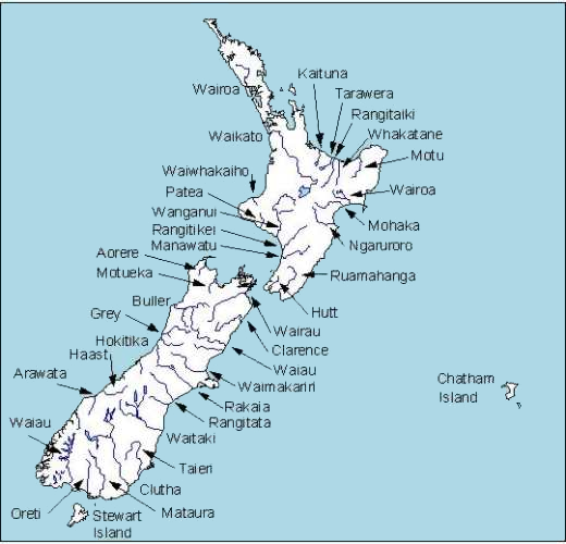 This is just scratching at the surface of the hydrological richness of Aotearoa though. Check out the resolution that the NZ Water Model is capable of giving us (Collins, D. and Zammit, C. Climate change impact on agricultural water resources and flooding. Prepared for the Ministry of Primary Industries. Client Report 2016114CH)! 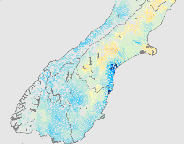 The NZ Water Model will be run using the output from the NZRCM, thus enabling the additional resolution of e.g. mountains to assist in predicting how global climate change will ultimately impact our local climate and hydrology. 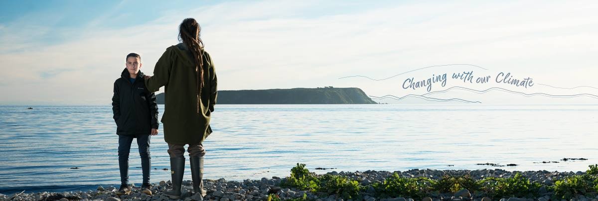 This has been a whistle stop tour of the modelling capability that we now have in place!
Keep an eye on our progress at the new and improved Deep South Challenge website. Firstly, a tribute to BrettThis year we lost a towering figure in the weather and climate research community, Dr Brett Mullan. He was my boss and was in fact the first person I met here, since he picked me up from the airport on my arrival. This work is dedicated to his memory. 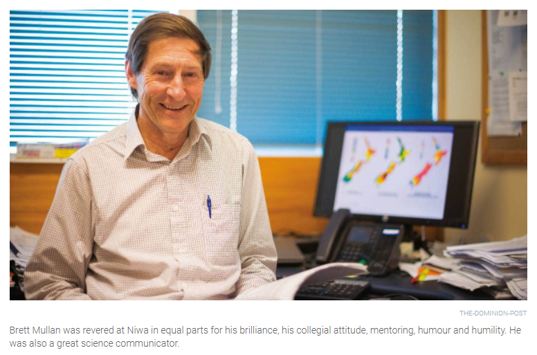 Image and caption from Brett's obituary by Susan Pepperell. Earth system modelling in the Deep South National Science ChallengeOne of the central deliverables of the Deep South National Science Challenge is the development of an earth system modelling capability to Aotearoa New Zealand. This model is now mature enough that its results are starting to appear in the peer-reviewed literature. There's also a recent blog post on the Deep South Challenge website about this from which I've taken the next image. 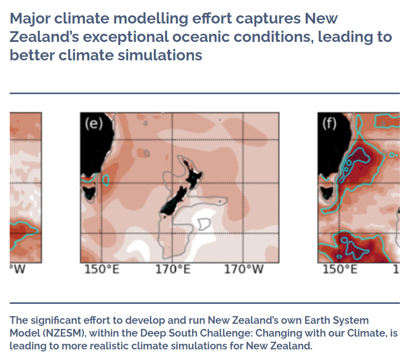 We are now at a very exciting stage in the model development where the global NZESM has produced 'hindcasts' from the mid 20th century up to 2015 as well as future climate change scenarios out to 2100. Clearly no one knows exactly what the future emissions pathways will look like and for this reason we have run 3 different future scenarios, which are shown here... 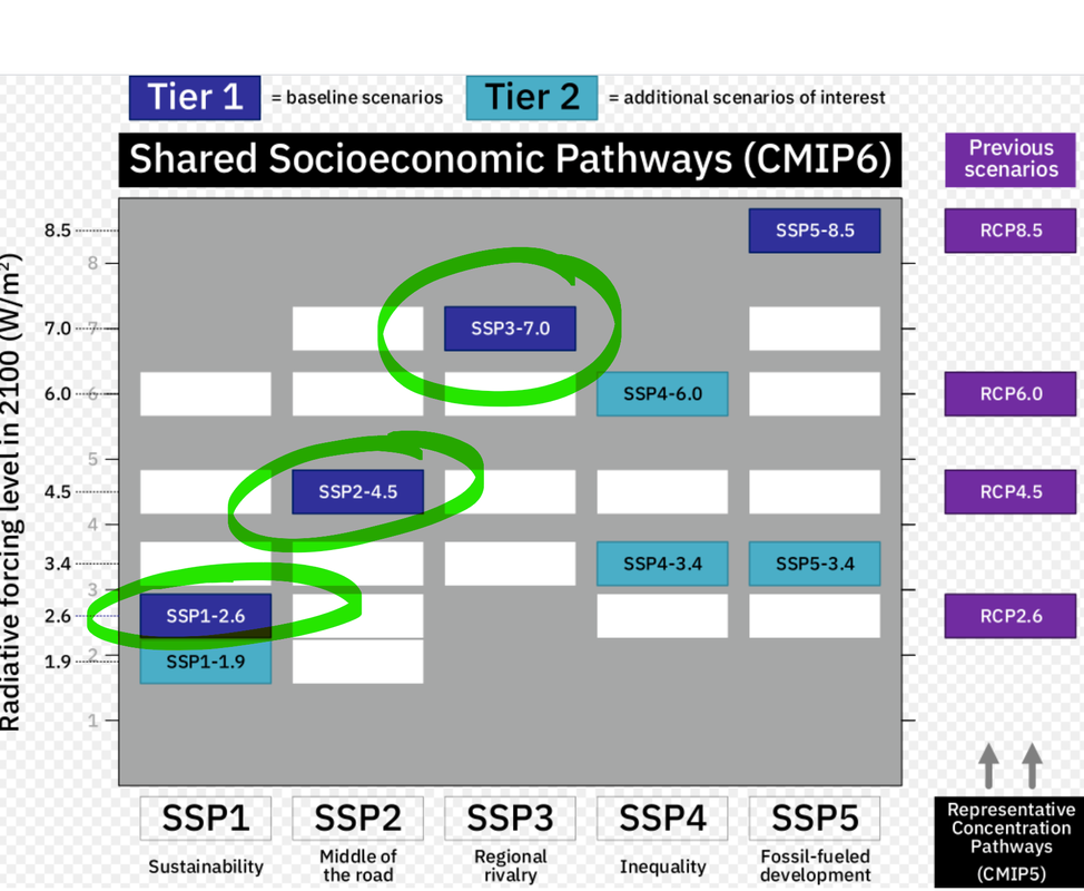 File:SSPs-CMIP6.svg. (2020, October 27). Wikimedia Commons, the free media repository. Retrieved 03:44, December 10, 2020 from https://commons.wikimedia.org/w/index.php?title=File:SSPs-CMIP6.svg&oldid=503215299. There are many of these scenarios and (for now) in this work we are only considering these 3. In their most basic forms: SSP1-2.6 is a low-emissions scenario, broadly consistent with the 'Paris Agreement' target of 2 degrees of warming; SSP2-4.5 is a medium emissions scenario and SSP3-7.0 models a high emissions (but not worst-case) future. Some of the aspects of the forcing of the model are illustrated here (from Meishausen et al.). 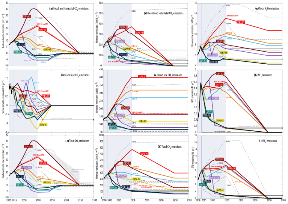 Since the NZESM is a global model, the resolution is fairly coarse. The next image shows the resolution of the global atmosphere component of the model. This shows air temperature near the surface and is clearly colder at the poles. Also note that the noisy coastline data is here is an artefact of the default options in the Ncview software used to (quickly) produce this figure! Incidentally, Ncview is free and brilliant for 'quick hacks' and producing animated gifs (using 'ncview -frames myfile.nc' and 'convert *.png mygif.gif'). 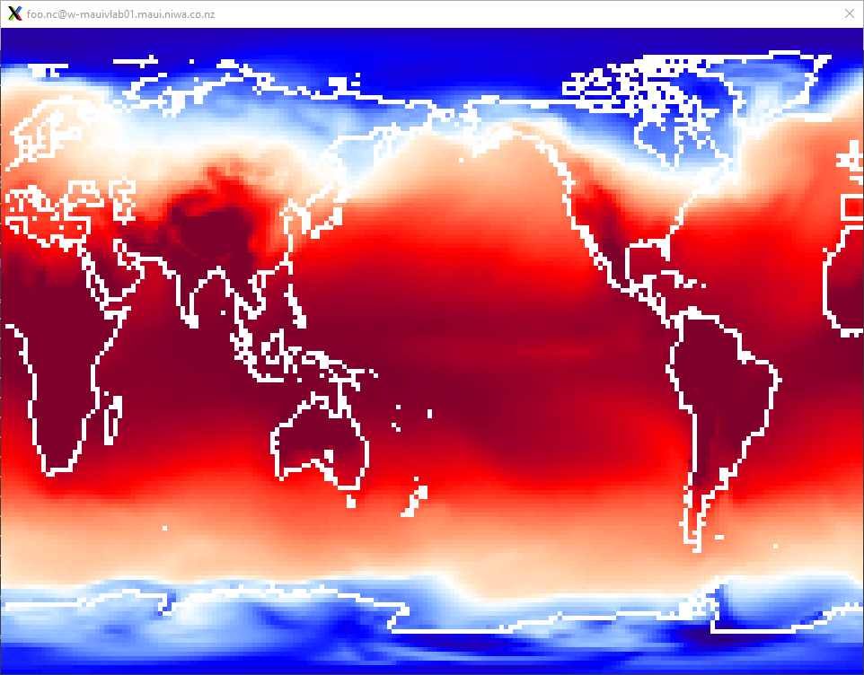 This figure is at the grid scale, which means that it is not smoothed. Now on a global scale this is fine, but if we zoom in to New Zealand...  ... we can see that the resolution is way too 'rough' to provide any meaningful regional information in a New Zealand context (again noting that the coastline data is an artefact; I just wanted to show the grid resolution). For example, in this resolution, Wellington, Nelson and Palmerston North would all be in the same or immediately neighbouring gridboxes. In the NZESM, as well as an atmosphere model, we have ocean, sea ice, ocean biogeochemistry and atmospheric chemistry too, all of which are able to change over time. In these senses, the NZESM is pretty much identical to its parent model, the UKESM. However, there are two main ways that the NZESM differs from the UKESM. Firstly it includes a solar cycle dependence of photolysis in the atmosphere and secondly, its major departure is the inclusion of a nested high resolution ocean model in the New Zealand region, as illustrated in Behrens at al., and here. 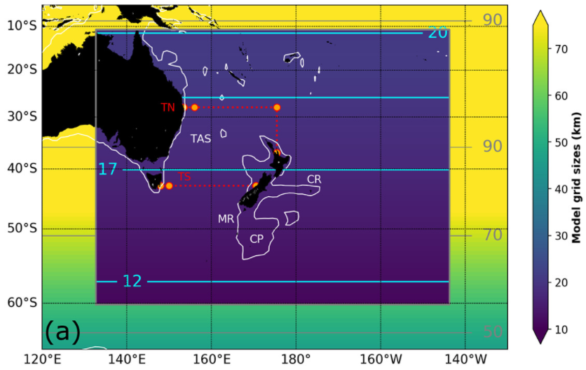 This big increase in ocean model resolution allows us to resolve eddies in the ocean which are not present in the global, lower resolution model. This image shows the sea surface height field of the ocean model in the two resolutions, just to show the gridscale resolution.  Here's a nifty animation I made of the sea surface height field using Ncview. This shows the ocean eddies which are able to transport heat south more efficiently, particularly via the East Australian Current.  Here's a final image of the sea surface circulation speed (again at the grid scale!). 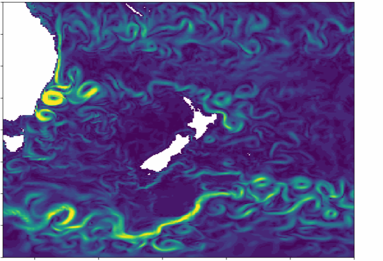 Because the atmosphere model in the NZESM is being forced from below by a higher resolution ocean, the atmospheric flows will be different.
We are currently performing a detailed analysis the output of the NZESM and the UKESM in detail to find out what differences the high resolution ocean around Aotearoa New Zealand predicts for our weather and climate in a changing world. We are also already generating data in a regional atmosphere climate model at 12km resolution, which is forced directly with raw data from the NZESM, and this in turn will feed into a catchment-scale hydrological model. Taken all together, this suite of work will provide global, national and regional scale climate and hydrological information to the scientific and policy-making communities in Aotearoa New Zealand. Watch this space! I'd really recommend this 'ultimate' .vimrc file if you're a Vim user... github.com/amix/vimrc I have forked it here... github.com/jonnyhtw/vimrc 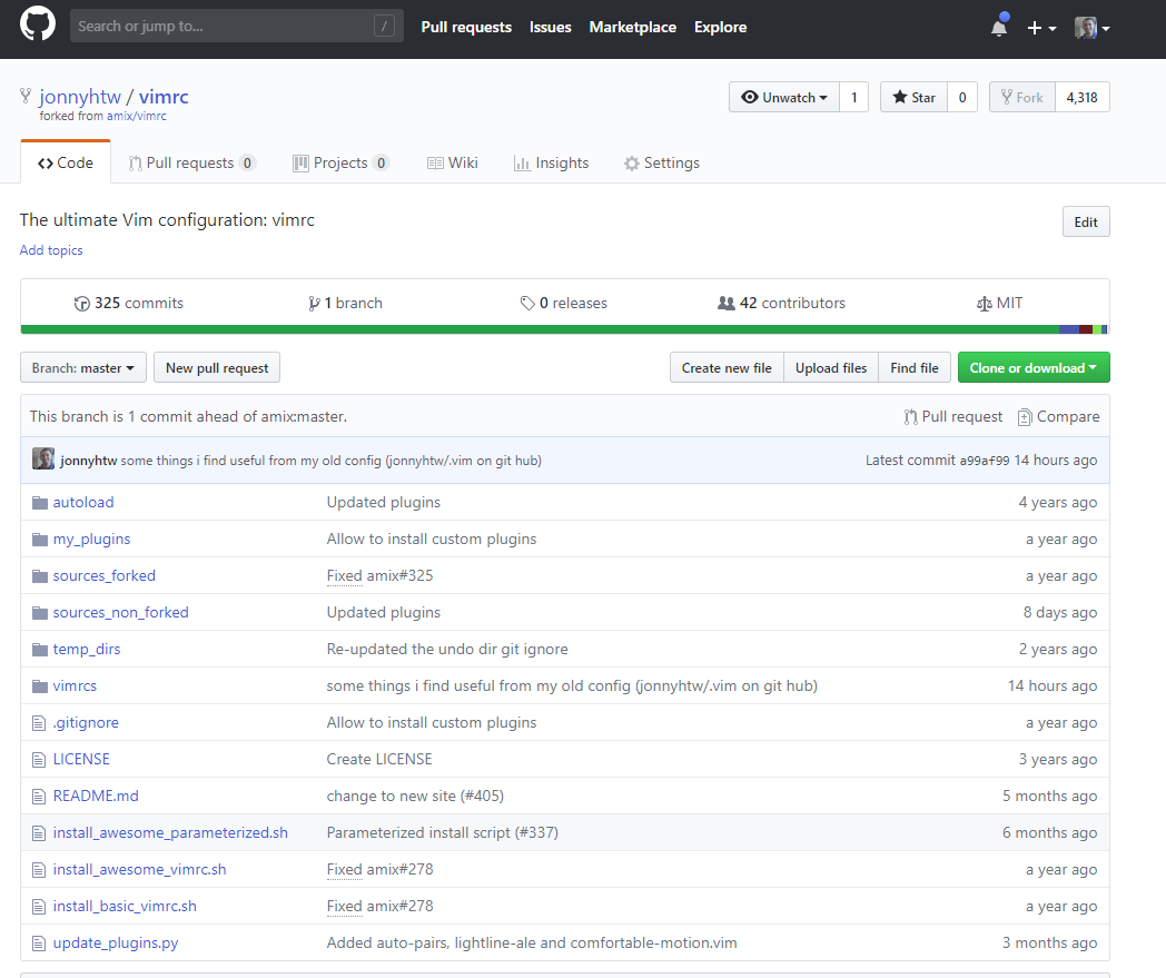 I've also made a few very minor changes to open splits on the right and the bottom respectively and always include line numbers. I've also mapped vimdiff 'diff searches' from [c to [ and ]c to ], just for ease! Enjoy! 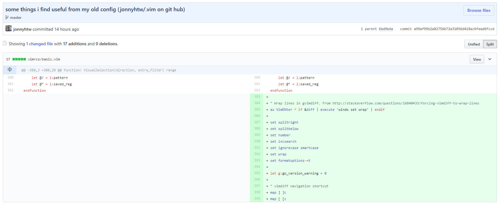 I'm doing some playing with the built in Veros examples and one of them is this amazing high res north Atlantic regional model... 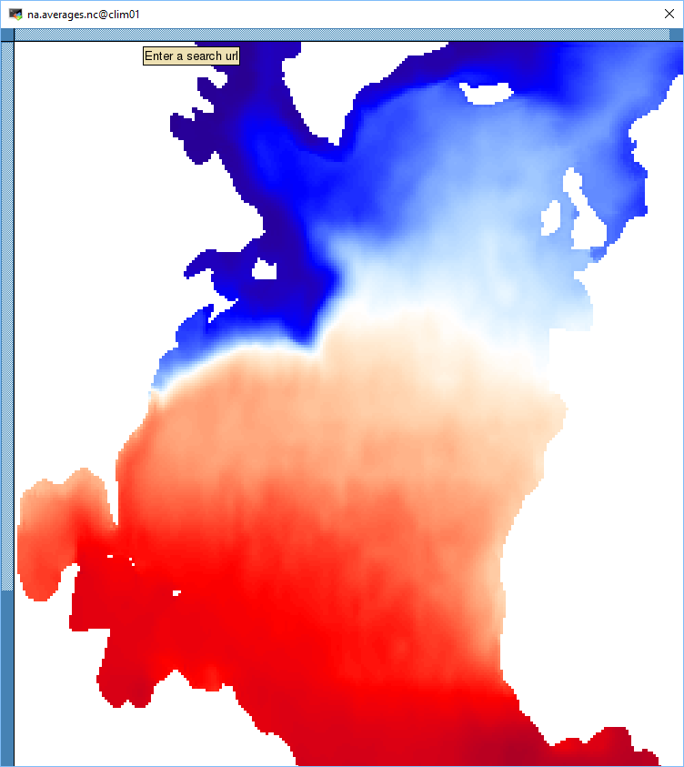 The redder colours are warmer water and the bluer ones are colder water.
See the discussion paper on Veros for more information! https://www.geosci-model-dev-discuss.net/gmd-2018-3/ A few months ago I posted about using the Veros ocean model, which is written in 'pure Python'. I have finally managed to find some time to get back to this and have produced a nice little gif (well, screen grab of one) of surface ocean circulation using the built in 4 degree global ocean example. The animated gif isn't here because you can't put gifs larger than 10MB on the free Weebly version! 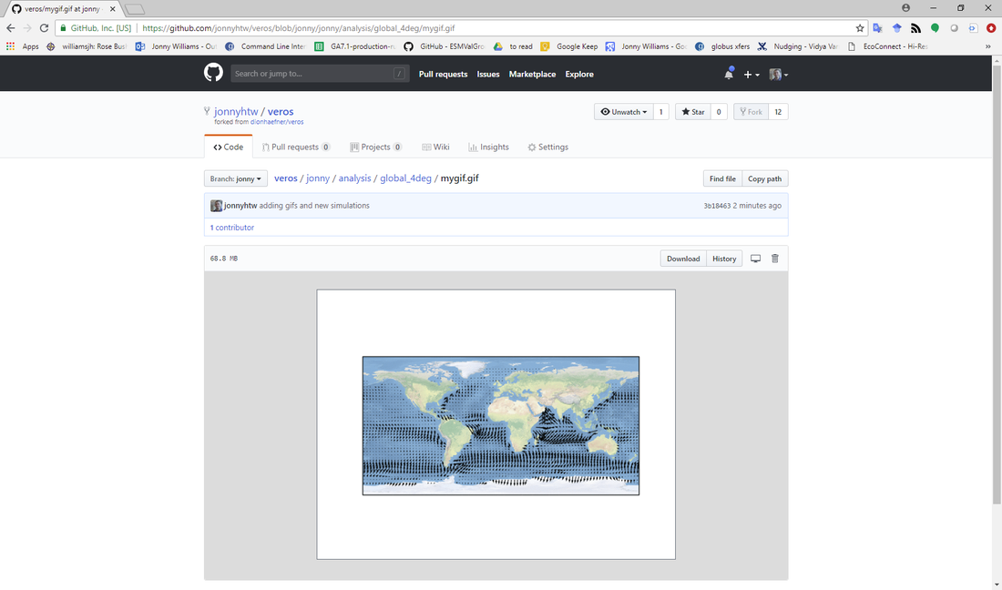 No scale, units or anything else at the moment but I'll get there eventually... ;)
I'll try and post more regularly from now on! Enjoy! 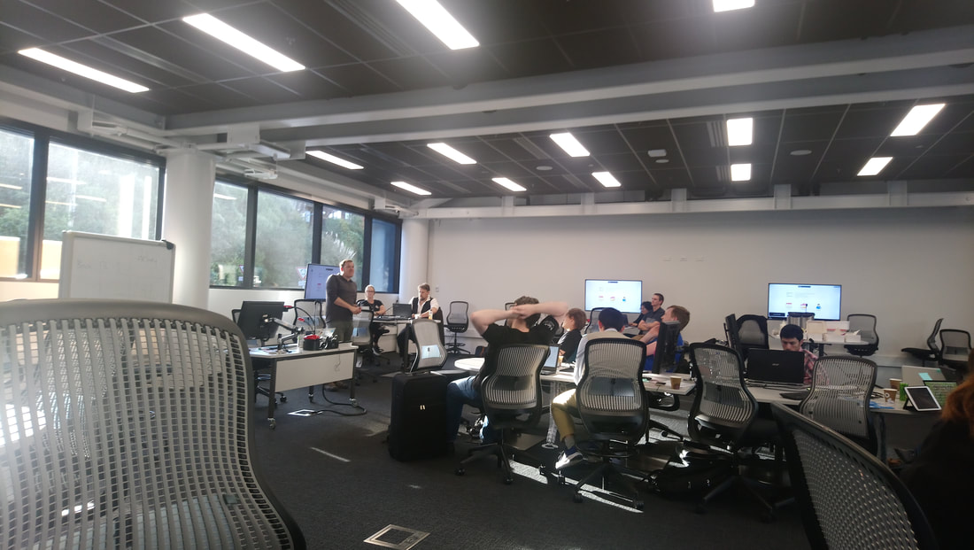 Jonah Duckles doing some instructing! Last week I undertook software Carpentry instructor training. This is something that I have wanted to do for a long time and I was very lucky to be able to do this at Victoria University of Wellington in my home city. 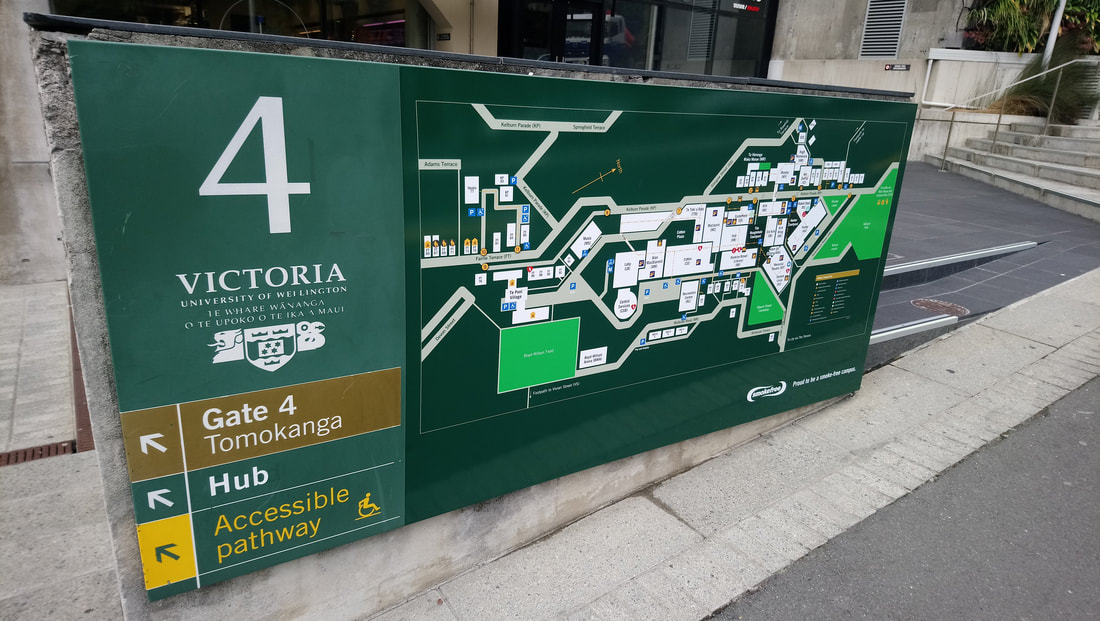 Arriving at class Software Carpentry is a global movement to educate people in techniques that will help them create better software. Link here. There are also library and data Carpentry training workshops which are now collectively known as 'the carpentries', carpentries.org/. A real emphasis is on training irrespective of personal work area though and the idea that librarians, bioinformaticians, social scientists and people just like me can all get this training is really empowering.  Fantastic facilities at the brand new Te Toki a Rata building at Victoria University of Wellington Software Carpentry itself is broadly split into three strands; controlling a computer environment using the ‘shell’ (sometimes called the command line or terminal), scientific computer programming with Python or R, and version control. 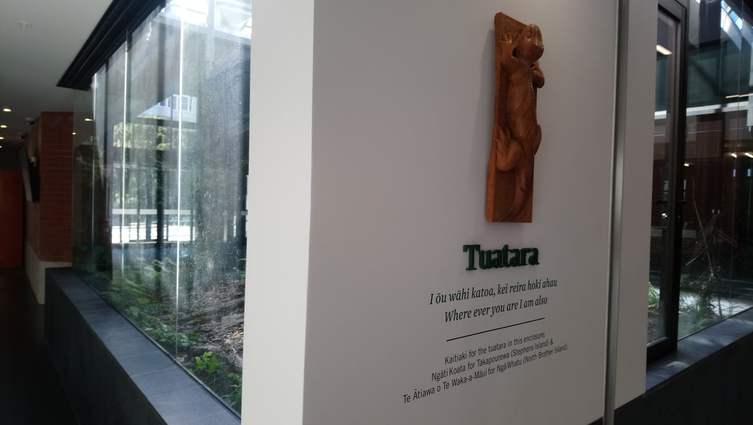 The tuatara enclosure right next to the teaching room. Sadly I didn't see any! The training itself was largely pedagogical (that is, learning to pass learning on to others) and this was quite new to me. We covered everything from working memory and cognitive load to live coding practice and how to organise a software carpentry workshop and everything in between. All of the materials are available on GitHub here carpentries.github.io/instructor-training/. 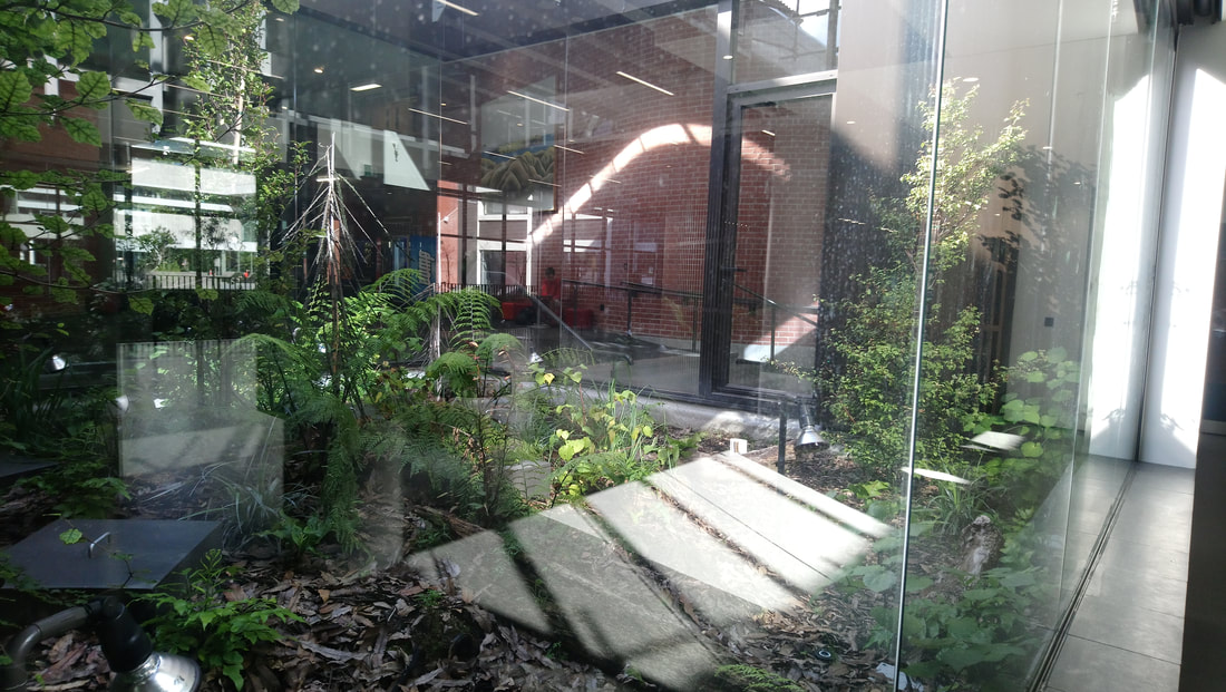 Hiding or sleeping tuatara? For me what I found by far the most challenging, was preparing and the presenting a short teaching session which was (shock horror) filmed and then played back to you in small groups. I was amazed at the effectiveness of this approach since it was rapid fire and then repeated so that we could progress in light of what we personally thought of our performance whilst also taking the thoughts of our other group members into account. I chose the shell as my teaching vehicle and it was incredible how quickly I descended into some jargon even though I tried not to! I believe that I improved during the course but I will find out how successful I was when I have to do a live demo of this to other people in the software Carpentry community online as part of my post course assessment. Wish me luck! 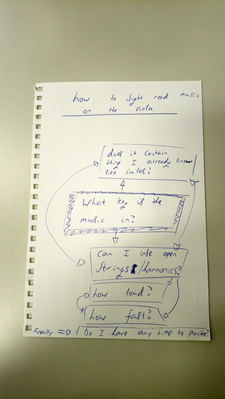 An example of a thought process that I frequently use outside of work, used as a method of illustrating pedagogy As a side note, something that I hadn't used before was etherpad (etherpad.org/). This is a way of collaborating online in real time with others in a group where everyone's input is colour coded, editable and open access. I'd recommend you give it a go. I will certainly be using is again in the future.  Great views of the city as I walked to Victoria University of Wellington An fantastic aspect of the software carpentry movement is the emphasis on the code of conduct., docs.carpentries.org/topic_folders/policies/code-of-conduct.html This ensures protection from discrimination and intimidation, whether conscious or otherwise in the instructor training and also in the courses which I will hopefully contribute to as a qualified instructor in the future. We all have aspects which make us different from the person metaphorically or physically next to us and so the knowledge that students and instructors are free to be themselves in a safe space is of comfort to me and I'm sure to many others also. I recently went to a conference where a similar code of conduct was expected of delegates and personally I found that just knowing that it was there made me feel empowered to be myself which boosted my confidence to be myself and be a better scientist and communicator.  Some better lighting here! Although I've been using Linux and shell based programming for about 14 years now, I never had any specific training in the style of software carpentry or actually anything remotely resembling it! I can confidently say that I would've programmed more efficiently, not deleted so many things accidentally, and saved myself and my fingernails a huge amount of pain via creating version controlled repositories and by writing better, more collaborative code!  The sun finally showed its face I very much hope to qualify soon to be a fully fledged software Carpentry instructor soon so that I can pass whatever knowledge I have to others in the ever growing community that I'm proud to be a little part of.
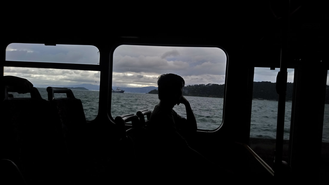
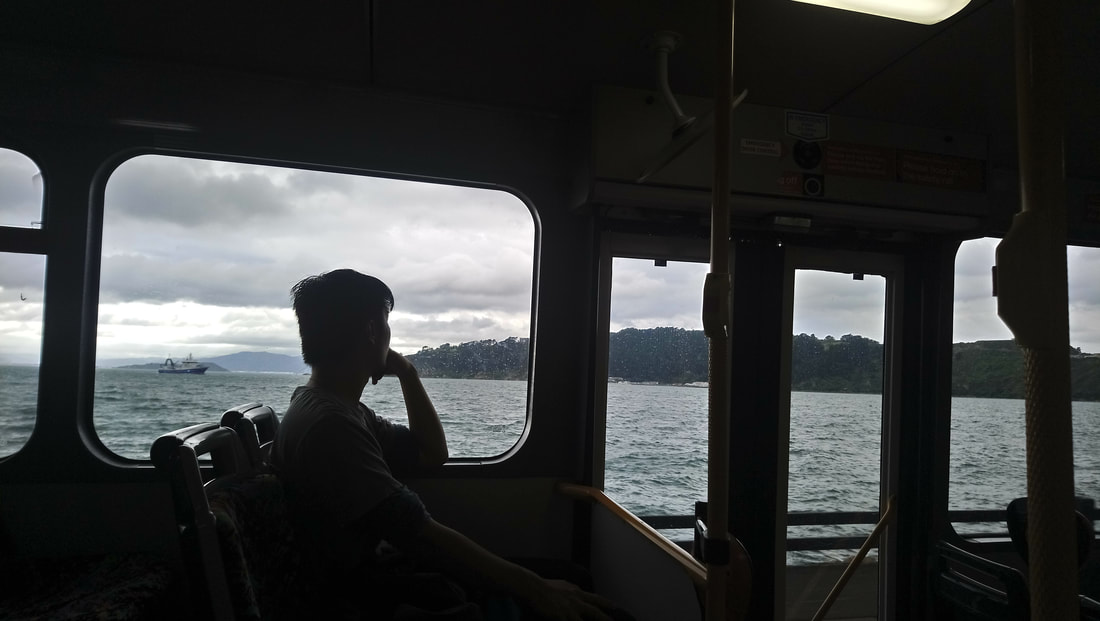
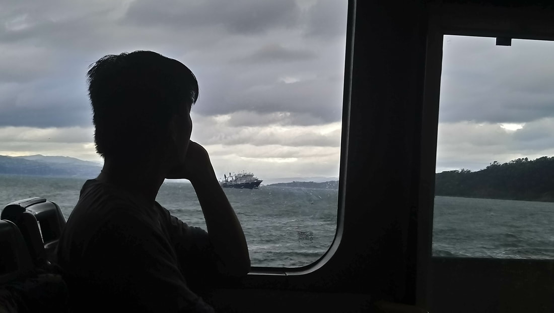
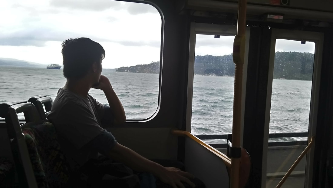
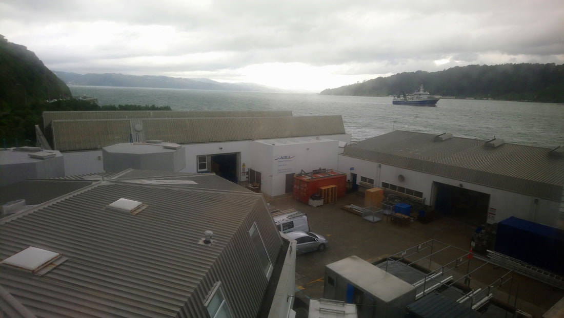
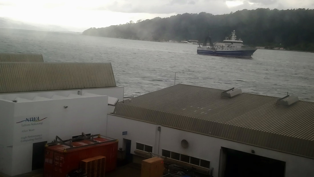
Does it work?! Ok let's try adding a photo I just took whilst waiting for the bus which never turned up... 🚌  Here's some pics I took last month on my way to work of the Tangaroa (our flagship research vessel) returning to Wellington after her latest Antarctic voyage! You can find out more about the journey here... https://www.niwa.co.nz/our-science/voyages/antarctica-2018. Happy Easter! Just a very quick post about the versatile ocean simulation package, Veros. I've only just started using it but it seems very cool. I've already run some models on Linux and using Mac OSX and it almost entirely works out of the box. More information is at the model's GitHub... http://veros.readthedocs.io/ here's some screen grabs from there... 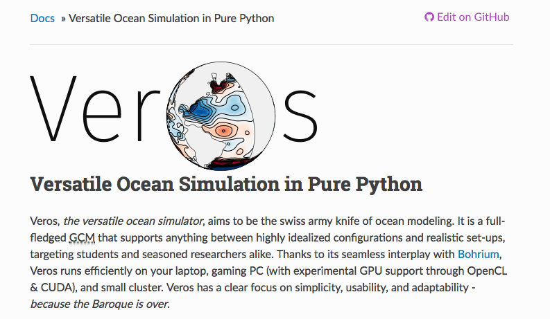 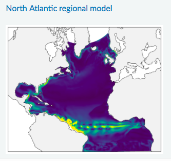 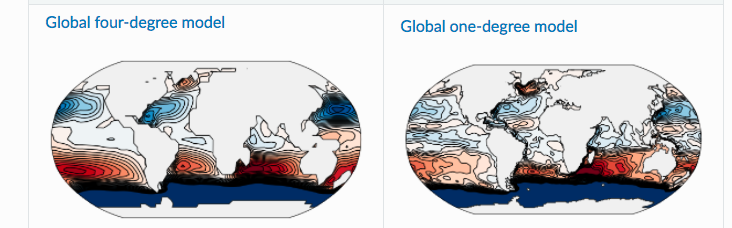 I'm looking forward to getting involved and have already been in touch with the lead developer regarding installation and its dependencies on the Python 'requests' package (http://docs.python-requests.org/en/master/). This has already resulted in a code change on GitHub! :)  |
AuthorThoughts on weather, climate, software dev, Python, open source and the like. Views are my own. 
Archives
March 2022
Categories
|


 RSS Feed
